Learning Accurate ML Explanations with Real-X and Eval-X
How do we efficiently generate ML explanations we can trust?
Machine learning models can capture complex relationships in the data that we as humans cannot. Perhaps there is a way to explain these models back to humans in order to help humans make high stakes decisions or learn something new.
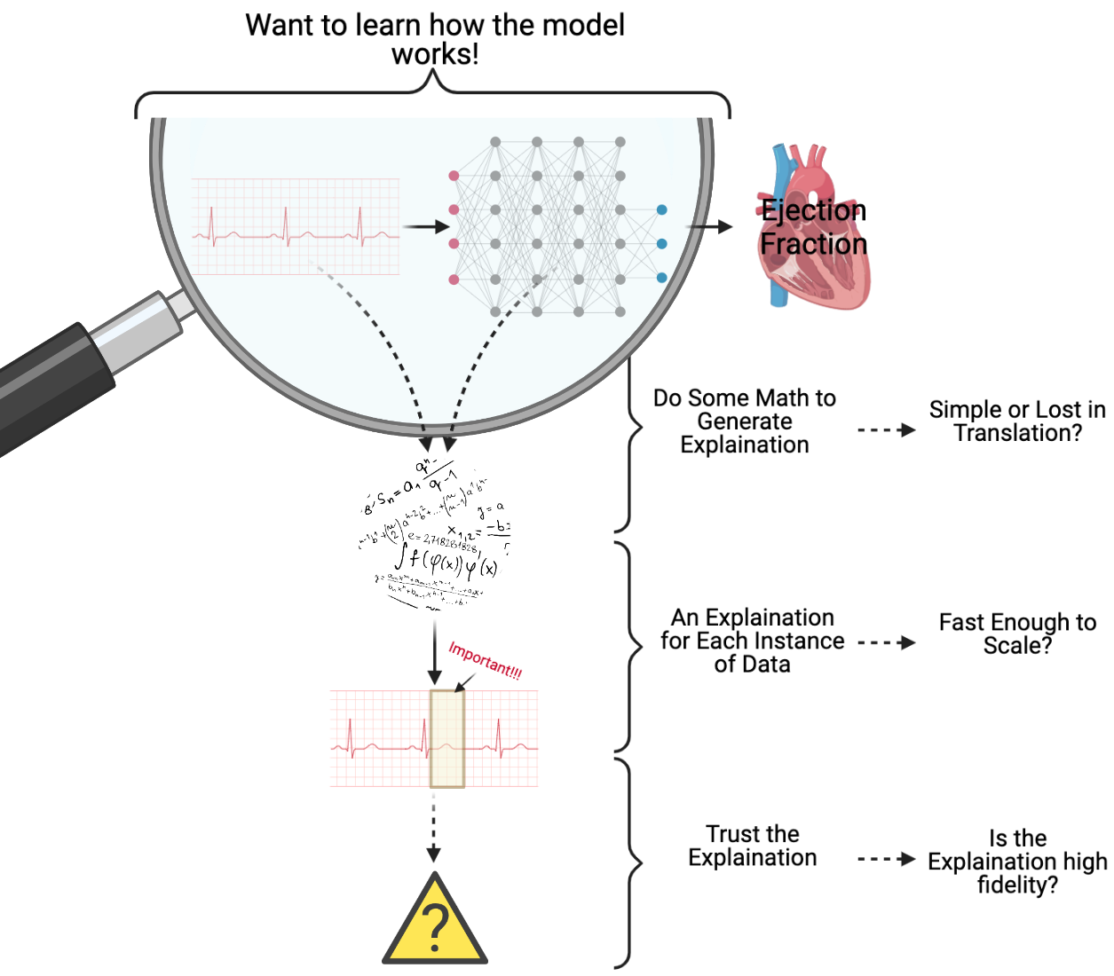
When I was working on estimating ejection fraction (a measure of how well the heart pumps blood) using patient electrocardiograms (ECGs), we wanted to understand how our machine learning model was able to estimate ejection fraction. I was told that physician’s wouldn’t be able to make such an estimation from ECGs alone, and I thought that if we could explain which parts of the ECG were influencing the model’s decision, then together we could uncover something new. However, when attempting to explain my model/data, I ran into a few problems, which I have attempted to capture in the figure below.

Firstly, ECGs are highly variable and complex, so we needed unique, personalized explanations for each ECG, which was not a quick process. However, my biggest issue was that I was in unknown territory and couldn’t be sure if any of the explanations generated were reasonable or could be trusted. Trusting the model was important, but trusting the explanation was even more important.
As pictured above, explanations identify which regions of the ECG are “important” using some mathematical operation. However, I wasn’t sure if these mathematical operations could be translated into something clinically relevant. For example, are large gradients for certain regions of the ECG clinically significant? Further, does the data support, with high fidelity, the conclusion that the important regions identified by the explanation method drive the estimation of ejection fraction?
Why Do We Need Interpretability in Machine Learning?
Data is complicated. Often it is difficult to make sense of complex patterns in the data, because the process by which it is generated remains unclear. Instead, practitioners have turned to machine learning to help model these mechanisms. Unfortunately, ML models are often too complex to understand.
In medicine, we are beginning to see ML models perform tasks that physicians cannot.
For example, as discussed, estimating estimating ejection fraction using ECGs
It’s natural to then ask…
What is an Interpretation/Explanation?
At a high level, explanations aim to provide users with an idea of what information is important for generating the model’s prediction or the target of interest.
One of the most active area of research in ML interpretability looks to provide users with explanations for a single prediction/target, by scoring the influence of each feature in the input. However, it is important to consider what these scores mean when translating them to an explanation.
Each interpretability method defines some mathematical operation, which provides their definition of interpretability.
For example, take gradient-based explanations.
Many of these, estimate the gradient of the prediction/target with respect to the input.
Roughly, the gradient estimates how that model’s output may change under very small perturbations to the input.
While, this may be useful, it is important to note that this is different from the identification of which features are the most important for generating the prediction/target.
Recent work has shown this empirically
Now let’s answer…
What Do We Want in an Explanation?
Physicians, for example, need to be able to make quick, accurate decisions in order to treat patient’s effectively. Based on our experience working with ECGs, we complied the follow list of wants, alluded to in the figure above:
- Instancewise (aka Personalized)
- We want instancewise explanations for multiple reasons. Firstly, our data may be translationally invariant. For example, we may be interested in identifying cancer from histology images. Here, our explanation should identify cancerous cells regardless of their location within the image. Secondly, instancewise explanations allow for a more granular understanding of the data. In medicine, this may help provide personalized information.
- Accurate/ High Fidelity
- We want explanations that can reliably provide which features are the most important for generating the model prediction/target.
- Simple
- We want explanations that are simple enough to be interpreted by a human, both in terms of their presentation to a human and the mathematical concept conveyed by the explanation.
- Fast
- Providing a granular/personalized understanding of the data can be computationally challenging, however it allows for a more dynamic insights to be gained. Therefore, we want to be able to provide explanations that scale to large datasets and can be accessed in real-time.
Now that we know we want…
Can We Have What We Want?
Let’s consider existing interpretability methods and break them into three groups:
| Gradient Based Methods | Locally Linear Methods | Perturbation Methods | |
|---|---|---|---|
| What? | Measure the gradient of output with respect to the input features? | Uses a linear function of simplified variables to explain the prediction of a single input | Perturb the inputs and observe the effect on the target |
| Examples | gradCAM |
LIME |
Occlusion |
| Why (not)? | Explanations don’t optimize for accuracy/fidelity. Recent work shows estimates of feature importance often do not identify features that help predict the target |
These methods are slow, requiring numerous perturbations of the input and/or training a new model per explanation. These perturbations may evaluate models where they are not grounded by data. | These methods are slow, requiring numerous perturbations to generate a single explanation. These perturbations may evaluate models where they are not grounded by data. |
Of note, both locally linear and perturbation-based methods rely on removing or perturbing features in order to characterize how/if the model’s prediction degrades. While removing important features may affect the prediction of the model, so too can the artifacts introduced by the removal or perturbation procedure.
While we can think of reasons to use each of these methods, none of them seem to satisfy our list of wants, either because they lack fidelity to the data or are too slow to scale to large datasets.
Is There Another Way?
Recently, Amortized Explanation Methods (AEM)
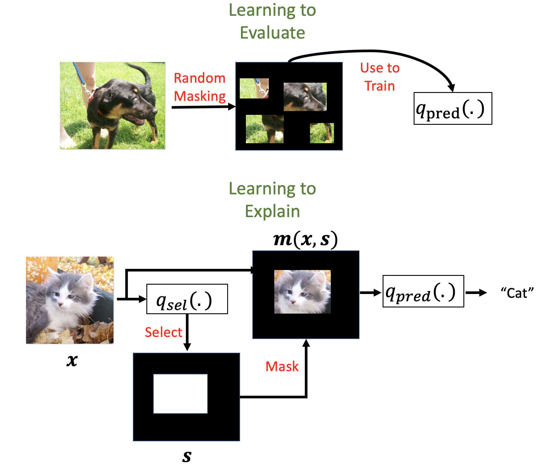
Let’s look at the following illustration, which exemplifies an amortized explanation method :

Here the selector model ($q_{\text{sel}}$) plays a simple game where it tries to select features which allow the predictor model ($q_{\text{pred}}$) to predict the target. This game aims to maximize the fidelity of the explanations directly. This game is captured by maximizing the follow amortized explanation method objective:
\[\mathcal{L}_{AEM} = \mathbb{E}_{x, y \sim F}\mathbb{E}_{s \sim q_{\text{sel}; \beta}(s \mid x ; \beta)}\left[\log q_{\text{pred}}(y \mid m(x, s) ; \theta) - \lambda R(s) \right].\]Here selector model ($q_{\text{sel}}$) is optimized to produce selections $s$ that maximize the likelihood of the masked data $\log q_{\text{pred}}(y \mid m(x, s) ; \theta)$. Then in order to ensure that the explanation is simple (presents a small set of important features) the objective pays a penalty for selecting each feature, expressed as $\lambda R(s)$.
You might be thinking…
What’s the Catch?
Well, first we have to choose the predictor model. We can either use an existing prediction model, which may not work well with the artifacts introduced by the masking process (i.e. occlusion to 0.) text, or train a new model, which requires care.
A few popular joint amortized explanation methods (JAMs) such as L2X
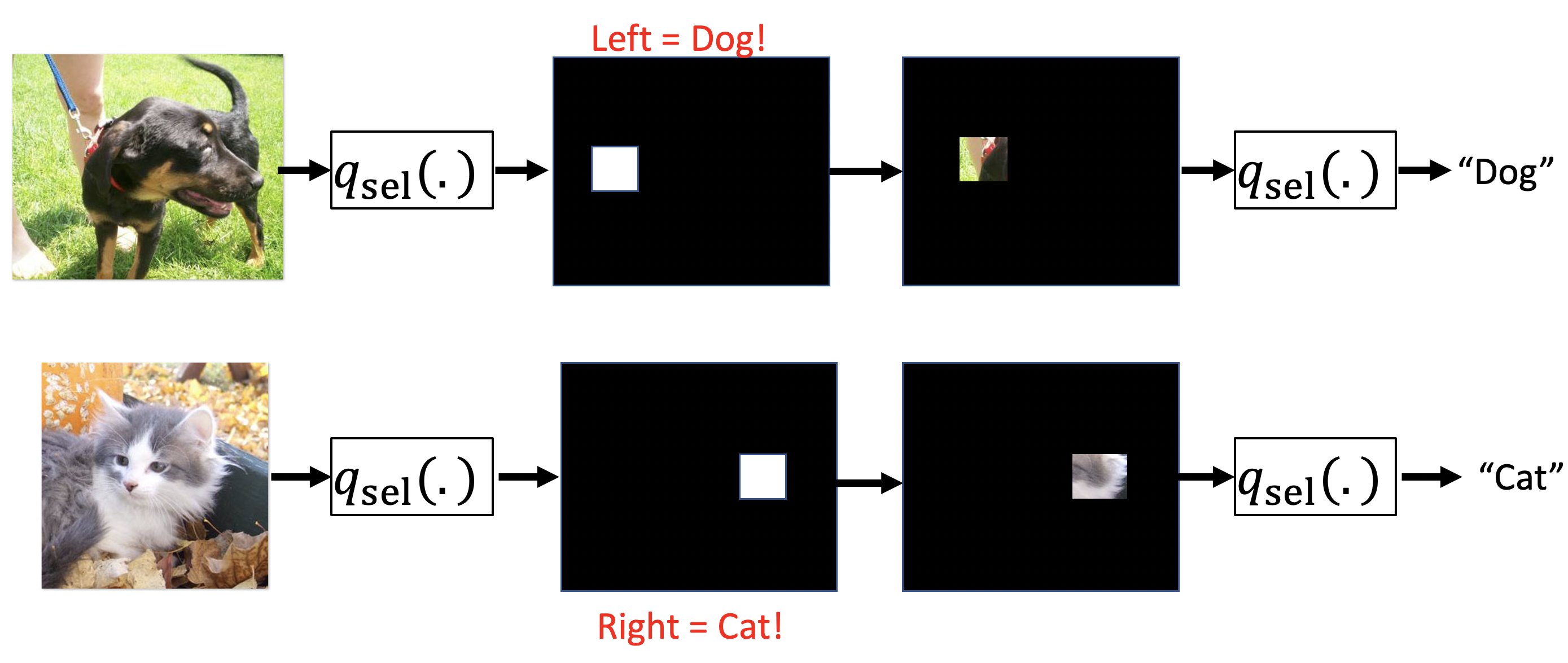
Let’s take a look at how this can go wrong:

In the above example, we see that these joint amortized explanation methods can learn to encode predictions. Here the selector model can select a pixel on the left to indicate dog and select a pixel on the right to indicate cat. Because the predictor is trained jointly, it can learn these encodings. Now, remember that the objective penalizes us for each pixel/feature selection. This encoding solution allows for accurate predictions with just a single pixel selection, helping to maximize the amortized objective.
Presented strange explanations like this in clinical settings can lead physicians to quickly loose trust. We need a way to validate the fidelity of the explanations.
Can We Evaluate the Explanations? (Eval-X)
Well, first we have to choose an evaluator model with which to evaluate the subset of important features identified by the interpretability method. We can either use an existing prediction model, which may not work well with the artifacts introduced by the masking process (i.e. occlusion to 0.), or train a new model, which requires care.
Are you getting de-ja-vu?
Popularly, RemOve And Retrain (ROAR)
Instead, we recently introduced Eval-X. Lets look at how Eval-X works.

Eval-X works by training a new evaluation model to approximate the true probability of the target given any subset of features in the input. Eval-X adopts a simple training procedure to learn this model by randomly selecting features during training. This procedure exposes the model to the same masking artifacts it will encounter during test time and ensures that the model cannot learn encodings.
Real-X, Let us Explain!
Given that Eval-X is robust to encodings and out-of-distribution artifacts, you might be wondering… is there a way use this approach to create a new amortized explanation method? Accordingly, we recently introduced Real-X, a novel amortized explanation method! Lets look at how Real-X works. (more de-ja-vu)

Real-X works by first training a new predictor model to approximate the true probability of the target given any subset of features in the input using the same procedure as Eval-X. Real-X then trains a selector model to select minimal feature subsets that maximizes the likelihood of the target, as measured by the Eval-X style predictor model. This prevents the selector model from learning encodings.
Real-X accomplishes the following:
- Provides fast explanations with a single forward pass
- Maximizes explanation fidelity/accuracy
- Provides simple explanations by selecting the minimal set of important features.
Do Real-X and Eval-X Really Work?
Before we can even think about using Real-X and Eval-X in the clinic we need to test the following claims:
- Real-X provides fast explanations without encoding
- Eval-X can detect encoding issues
To do so, lets see how Real-X stacks up against other amortized explanation methods and whether or not Eval-X can detect encodings. Well take a look at:
- L2X (Learning to Explain)
- INVASE
- BASE-X (Copies Real-X score function gradient estimation technique REBAR, but is a an amortized explanation method that learns the selector and predictor models jointly)
- FULL = A model trained on the full feature set.
To make the comparison concrete, our goal is to provide simple explanations by selecting as few features as possible while retaining our ability to predict.
Evaluation:
Each amortized explanation method we consider first makes selections, then uses those selections to predict the target using is predictor model. The predictive performance of the amortized explanation method is supposed to provide us with a metric of how good the explanations are. We’ll consider the following metrics: area under the receiver operator curve (AUROC) and accuracy (ACC).
We’ll also look at the predictions that Eval-X produces given each method’s explanations. Let’s denote these metrics with a prefix “e”: eAUROC and eACC.
If the amortized explanation method is encoding, then we would expect high AUROC/ACC and low eAUROC/eACC.
Now lets see how well each method is able to explain Chest X-Rays.
Cardiomegaly Classification from Chest X-Rays
Cardiomegaly is characterized by an enlarged heart and can be diagnosed by measuring the maximal horizontal diameter of the heart relative to that of the chest cavity and assessing the contour of the heart. Given this, we expect to see selections that establish the margins of the heart and chest cavity.
We used the The NIH ChestX-ray8 Dataset
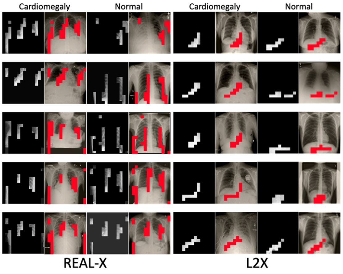
Let’s take a look at some randomly selected explanations from each method.


An initial review of these samples suggests that L2X, INVASE, and BASE-X may be making some selections that don’t appear to establish the margins of the heart, the margins of the chest wall, nor the contour of the heart. Real-X on the other hand appears to be in line with our intuition of what should be important. However, we can’t be sure without additional evaluation.
Now, lets take a look at the in-built and EVAL-X evaluation metrics:

All the explanation methods provide explanations that are highly predictive when assess directly by the method. However, Eval-X is able to reveal that L2X, INVASE, and BASE-X are all encoding the predictions in their explanations, achieving eACC ~50%. Meanwhile, the sections made by Real-X remain fairly predictive when evaluated by Eval-X.
Finally, let’s look at what two expert radiologists thought of the explanations generated by each method.
We randomly selected 50 Chest X-rays from the test set and displayed the selections made by each method for each X-ray in a random order. The radiologists ranked the four options provided.

From this, we see that the physicians tended to choose the selections generated by Real-X.
How to Implement Real-X?
Explaining with Real-X involves three steps:
- Initialize the selector model and predictor model. (Any model architecture can be specified)
- Choose the Real-X hyperparameter (lambda) and any other training hyperparameters (i.e. batch_size)
- Train the predictor and the selector model.
Once Real-X can been trained, its selector model can be used directly to generate explanations. Real-X explanations can also be validated with Eval-X (built-in).
Please, check out our example to see how we apply Real-X to explain MNIST classifications.